---

Currently not logged in.

main | wiki | tasks | examples | forums | privacy | login

---

Analysis of transiting extrasolar planets

In this example, we demonstrate how the FITSH task can be used to completely reduce a data series acquired for a transit of the extrasolar planet HAT-P-13b. These observations were made on the night of 2010 December 27/28, between 23:21 and 04:28 UT using the 60/90/180 cm Schmidt telescope located on the Piszkés-tető Mountain Station of the Konkoly Observatory, Hungary. The nominal length of the transit of this planet is approximately 3.5 hours, and this series of observations were almost scheduled for the predicted mid-transit time, 01:49 UT (using the available ephemerides at that time). All in all, 460 individual frames were taken with a net exposure time of 20 seconds, thus one cycle was approximately 42 seconds (i.e. adding the 22 seconds of overhead yielded by the camera readout). See the paper Transit timing variations in the HAT-P-13 planetary system for more details about the physics of this planetary system (and where these measurements have been published shortly after this observation).

If you intend to try this set of data reduction scripts in your system, the full archive of related data can be downloaded by downloading the individual files listed here: hatp13-20101227.list. This archive includes the 460 calibrated frames, the base.list file containing the ``basenames'' of these frames, the projected catalogue centered around the target star HAT-P-13 and a script (named vizquery-hatp13.sh) that downloads and creates this catalogue using the cdsclient package (and the grtrans task). Note that this archive linked above is very large: the individual calibrated images have a size of 4096 × 4096 pixels, thus each image is approximately 64 megabytes (using 32-bit floating point representation), therefore the whole archive is around 30 gigabytes.

Data structures

Before starting the ``real'' data reduction, some directories should be created where the intermediate products (astrometric data, instrumental photometry and so on) are stored. These directories are referred symbolically (i.e. via shell variables) in the subsequent scripts, so in practice these can be arbitrary. Here in this example, we set up these directories as the subdirectories of the ``current'' directory. The calibrated FITS images are also put into one of these subdirectories, namely the one with the name of ./fits and referred as $FITS.

#!/bin/bash

# Copy FITS files here:
FITS=./fits;	test -d $FITS || mkdir -p $FITS

# Create these directories as well:
ASTR=./astrom; test -d $ASTR || mkdir -p $ASTR
REG=./reg    ; test -d $REG  || mkdir -p $REG
PHOT=./phot  ; test -d $PHOT || mkdir -p $PHOT

Star detection and initial astrometry

Prior to the photometry, the centroid coordinates of the target star HAT-P-13 (USNO 1373-0235571) and the comparison stars (USNO 1374-0234366, 1374-0234452 and 1376-0234158) have been computed by using the astrometric solutions for each image.

First, stars where searched using the task fistar, on the images shrunk by a factor of two (see also the constant $SHF). The resulted coordinates were then multiplied by two, using the program awk in order to have a proper set of coordinates on the original images as well:

#!/bin/bash

FITS=./fits
ASTR=./astrom

SHF=2

cat base.list | \
while read base dummy ; do

        if test 1 -lt $SHF ; then
                fitrans $FITS/$base.fits --shrink $SHF
        else
                cat     $FITS/$base.fits
        fi | \
        fistar  --input - \
                --flux-threshold 6000 --model elliptic \
                --format id,x,y,s,d,k,flux,mag \
                --output - | \
        awk -v s=$SHF \
         '{     print $1,$2*s,$3*s,$4,$5,$6,$7,$8;
         }' > $ASTR/$base.stars

        echo "$base: done." >> /dev/stderr
done

Here the original FITS images are supposed to be placed in the directory ./fits and the list of detected stars (files with the extension of *.stars) are put in the subdirectory ./astrom. The ``basenames'' of the original files are stored in the file base.list. These ``basenames'' are the names with the original FITS files without the *.fits extension.

Second, relative and absolute astrometic transformations were obtained by using the task grmatch. Here, we used a second order polynomial for the relative and a third order polynomial for the absolute astrometry.

#!/bin/bash

ASTR=./astrom

ref=Rhatp13-0201-I

cat base.list | \
while read base dummy ; do

        grmatch --reference hatp13.cat --col-ref 2,3 --col-ref-ordering -5 \
                --input $ASTR/$base.stars --col-inp 2,3 --col-inp-ordering -8 \
                --max-distance 1 \
                --order 3 --triangulation auto,unitarity=0.01,maxref=400,maxinp=400 \
                --weight reference,column=5,magnitude,power=2 \
                --comment --output-transformation $ASTR/$base.atrans

        grmatch --reference $ASTR/$ref.stars --col-ref 2,3 --col-ref-ordering -8 \
                --input $ASTR/$base.stars --col-inp 2,3 --col-inp-ordering -8 \
                --max-distance 1 \
                --order 2 --triangulation auto,unitarity=0.01,maxref=400,maxinp=400 \
                --weight reference,column=8,magnitude,power=2 \
                --comment --output-transformation $ASTR/$base.dtrans

        echo "$base: done." >> /dev/stderr
done

Refined astrometry

The problem with the above shown (and implemented) algorithm is since the task fistar might not have detected some of the stars, in some cases both the relative and absolute astrometric solutions might be systematically distorted. In order to overcome this problem, we do the following:

• First, create a high signal-to-noise image from the previous images.
• Second, using this high SNR image, we build an internal new catalogue that contains the projected or pixel coordinates of the stars and the USNO identifiers as well.
• Using this new catalogue, we refine the astrometric solutions by re-fitting the star centroids on all of the images.

Although this refined astrometry is not essential for these images (large field-of-view, several hundreds of stars with good detections), it is more relevant when the number of detected stars is significantly smaller (i.e. analyizing images of a telescope with a smaller FOV).

The high SNR image can be created by registering the individual images to the same reference system (using the *.dtrans initial relative astrometric solutions and the fitrans untility) and then using the task ficombine to average them:

#!/bin/bash

FITS=./fits
ASTR=./astrom
REG=./reg

for base in     Rhatp13-0190-I Rhatp13-0191-I Rhatp13-0192-I Rhatp13-0193-I Rhatp13-0194-I \
                Rhatp13-0195-I Rhatp13-0196-I Rhatp13-0197-I Rhatp13-0198-I Rhatp13-0199-I \
                Rhatp13-0200-I Rhatp13-0201-I Rhatp13-0202-I Rhatp13-0203-I Rhatp13-0204-I \
                Rhatp13-0205-I Rhatp13-0206-I Rhatp13-0207-I Rhatp13-0208-I Rhatp13-0209-I 
do
        fitrans --size 4096,4096 --input $FITS/$base.fits \
                --input-transformation $ASTR/$base.dtrans \
                -c --reverse --output $REG/$base.fits

        echo "$base: done." >> /dev/stderr
	
done

ficombine \
        $REG/Rhatp13-0190-I.fits $REG/Rhatp13-0191-I.fits $REG/Rhatp13-0192-I.fits $REG/Rhatp13-0193-I.fits $REG/Rhatp13-0194-I.fits \
        $REG/Rhatp13-0195-I.fits $REG/Rhatp13-0196-I.fits $REG/Rhatp13-0197-I.fits $REG/Rhatp13-0198-I.fits $REG/Rhatp13-0199-I.fits \
        $REG/Rhatp13-0200-I.fits $REG/Rhatp13-0201-I.fits $REG/Rhatp13-0202-I.fits $REG/Rhatp13-0203-I.fits $REG/Rhatp13-0204-I.fits \
        $REG/Rhatp13-0205-I.fits $REG/Rhatp13-0206-I.fits $REG/Rhatp13-0207-I.fits $REG/Rhatp13-0208-I.fits $REG/Rhatp13-0209-I.fits \
        --output hatp13.fits

Using this combine hatp13.fits image, we build the new catalogue:

#!/bin/bash

base=hatp13

fistar  ${base}.fits --flux-threshold 2000 \
        --model elliptic --format id,x,y,s,d,k,flux,mag \
        --output ${base}.stars

grmatch --reference ${base}.cat --col-ref 2,3 --col-ref-ordering -5 \
        --input ${base}.stars --col-inp 2,3 --col-inp-ordering -8 \
        --max-distance 1 \
        --order 3 --triangulation auto,unitarity=0.01,maxref=400,maxinp=400 \
        --weight reference,column=5,magnitude,power=2 \
        --comment --output-transformation ${base}.atrans --output ${base}.match

cat     ${base}.match | \
awk \
  '{     printf("%s %10.3f %10.3f %7.3f %7.3f %7.3f\n",$1,$8,$9,$4,$5,$6);
  }' > ${base}.list

This step above creates

• the file hatp13.stars with the list of raw star detections;
• the file hatp13.match and hatp13.atrans containing the list of matched USNO catalogue entries and the absolute astrometric solution;
• and the file hatp13.list, that is an excerpt from the hatp13.match file containing only the USNO identifiers and the X,Y pixel coordinates on the image hatp13.fits.

Now, exploiting this new ``local catalogue'' of hatp13.list, we refine the astrometry by involving fiphot to refine the star centroid coordinates on all positions found in the catalogue and then we use the task grtrans to fit a new relative astrometric transformation for these refined star profile centroid lists:

#!/bin/bash

FITS=./fits
ASTR=./astrom
REG=./reg

ref=Rhatp13-0201-I

(       echo    $ref
        cat     base.list 
) | \
while read base dummy ; do

        grtrans hatp13.list --col-ref 2,3 \
                --input-transformation $ASTR/$base.dtrans \
                --output - | \
        fiphot  $FITS/$base.fits \
                --input-list - --col-id 1 --col-xy 2,3 \
                --gain 1.00 --apertures 6:30:10 \
                --sky-fit median \
                --format IXY,XYxyFfM \
                --output $ASTR/$base.xstars

        paste   $ASTR/$ref.xstars $ASTR/$base.xstars | \
        grtrans --col-ref 4,5 --col-fit 14,15 \
                --order 3 --comment --col-weight 10 --weight magnitude,power=2 \
                --output-transformation $ASTR/$base.xtrans

	echo "$base: done." >> /dev/stderr

done

This final step of the refined astrometry created two series of files in the astrometry directory $ASTR, namely the files with the extension of *.xstars containing the refined stellar centroid coordinates and the files with the extension of *.xtrans containing the refined relative transformations.

Photometry

Photometry is then rather simple, i.e. we have to transform the local catalogue hatp13.list to each individual image using the refined relative transformations (the files $ASTR/*.xtrans) and perform the photometry with the task fiphot. The output of the photometry is collected in the directory $PHOT.

#!/bin/bash

FITS=./fits
ASTR=./astrom
PHOT=./phot

cat base.list | \
while read base dummy ; do

	grtrans hatp13.list --col-ref 2,3 \
		--input-transformation $ASTR/$base.xtrans \
		--output - | \
	fiphot  $FITS/$base.fits --input-list - --col-id 1 --col-xy 2,3 \
                --gain 1.00 --apertures 6:30:10,8:30:10,10:30:10,12:30:10,14:30:10 --disjoint-rings \
		--sky-fit median \
                --serial $base --format SIXY,MmBbFfs \
                --output $PHOT/$base.phot

	echo "$base: done." >> /dev/stderr

done

Light curves

The light curve of HAT-P-13 can be extracted from the $PHOT/*.phot files by simply searching the catalogue identifier of the target star and the comparison stars and subtract the respective magnitudes. However, if there are multiple comparison stars, the target magnitude can also be estimated by converting the magnitude values to fluxes, summing up the fluxes of the comparison stars and the converting the total flux to magnitude.

The tasks in the FITSH package does not provide any direct feature for this purpose, however, it can be implemented easily involving the awk programming language. The script below implements the algorithm described above in order to estimate the flux of the target star (HAT-P-13, 1373-0235571). Since aperture photometry is performed for not a single aperture but a series of these, one should specify the target aperture as well.

#!/bin/bash

function jd()
 {	echo $1 $2 $3 | \
	awk \
	 '{    y=$1;m=$2;d=$3;
	        if ( m <= 2 ) { y-=1;m+=12; }
        	jm=int(1461*y/4)+int(153*(m+1)/5)-int(y/100)+int(y/400);
	        j=jm+d+1720996.5;
        	printf("%.5f\n",j);
	 }'
 }

FITS=./fits
PHOT=./phot

RA=129.8833; DEC=47.3519

APERTURE=4
TARGET=1373-0235571
COMP=1374-0234366,1374-0234452,1376-0234158

n=1
cat base.list | \
while read base dummy ; do

        test -f $PHOT/$base.phot || continue

        date=`fiheader $FITS/$base.fits --get date-obs | tr "T:-" "   " | awk '{ printf("%s %s %.5f\n",$1,$2,$3+($4*3600+$5*60+$6)/86400); }'`
        jd=`jd $date`
        bjd=`echo $jd | lfit -c jd -f "bjd(jd,$RA,$DEC)" -F "%.5f"`

        cat     $PHOT/$base.phot | \
        awk     -v base=$base -v jd=$bjd -v T=$TARGET -v C=$COMP -v a=$APERTURE \
         'BEGIN \
          {     fc=0;
                nc=0;
                ncomp=split(C,comps,",");
          } \
        !/^#/{  id=$2;
                mag=$(4+7*(a-1)+1);
                err=$(4+7*(a-1)+2);
                bg=$(4+7*(a-1)+3);
                bs=$(4+7*(a-1)+4);
                if ( id==T )
		 {	m0=mag;
                        e0=err;
                        b0=bg;
                        s0=bs;
                 }
                else 
                 {      j=0;
                        for ( i=1 ; i<=ncomp ; i++ )
                         {      if ( comps[i]==id )     j=1;    }
                        if ( j>0 )
                         {      fc+=exp(-mag*log(10)/2.5);
                                nc+=1;
                         }
                 }
         } \
        END \
         {      mc=-2.5*log(fc)/log(10);
                mag=m0-mc;
                err=e0;
                printf("%10.5f %9.5f %9.5f %s\n",jd,mag,err,base);
         }'

        n=$((n+1))

done > hatp13.lc 

Note that the FITS package does not have a built-in JD (Julian Day) conversion routine, so the jd() shell function at the beginning of the script implements this neccessary functionality. The JD to BJD conversion is done by the task lfit.

Light curve modelling

Once the final light curve is ready for this observation, that is created by the above script in the file named hatp13.lc, we can analyize the results using also the task lfit. This program has some built-in features that aids the analysis of photometry from transiting extrasolar planets.

#!/bin/bash

function mean_motion()
{
 echo $1 | awk '{ printf("%.7f\n",4*atan2(1,0)/$1); }'
}

function lfit_funct_tlc()
 {
  echo  -x "zcorr(ph)=1-ph^2" \
        -x "ycorr(ph)=1-ph^2/3" \
        -x "lcbase(p,b2,om,dt)=ntiq(p,sqrt(abs(b2)*zcorr($n*dt)+(1-abs(b2))*(om*dt)^2*ycorr($n*dt)),$G1,$G2)" 
 }

function lfit_funct_magnitude()
 {
  echo  -x "magflux(f)=-2.5*log(f)/log(10)" \
        -x "fluxmag(m)=exp(-0.4*m*log(10))"
 }

P=2.91626
n=`mean_motion $P`

G1=0.2785       # I-band
G2=0.3273       # I-band

E=2455558.57121
om=17.070
p=0.0844
b2=0.447

mag0=0.910

base=hatp13

epd="(mag0+mag1*(t-$E)+mag2*(t-$E)^2)"

lfit     $base.lc \
         `lfit_funct_tlc` \
         `lfit_funct_magnitude` \
         -v E=$E,p=$p,b2=$b2[0:1],om=$om,mag0=$mag0,mag1=0,mag2:=0 \
         -F E=%13.5f,p=%6.4f,b2=%5.3f,om=%6.3f,mag0=%8.5f,mag1=%8.5f,mag2=%8.5f \
         -c t:1,mmag:2,merr:3 \
         -f "$epd+magflux(lcbase(p,b2,om,t-E))" \
         -y mmag \
         -e "(merr*1.45)*1.05" \
         --xmmc --iterations 1000 \
         --output $base.xmmc

A=($(cat $base.xmmc | grep -v "^#" | head -n 1))

lfit    $base.lc \
        `lfit_funct_tlc` \
        `lfit_funct_magnitude` \
        -v E=${A[0]},p=${A[1]},b2=${A[2]},om=${A[3]},mag0=${A[4]},mag1=${A[5]},mag2=${A[6]} \
        -c t:1,mmag:2,merr:3 \
        -f "t,mmag-$epd,merr,magflux(lcbase(p,b2,om,t-E)),(mmag-$epd)-magflux(lcbase(p,b2,om,t-E))" \
        -F %13.5f,%9.5f,%9.5f,%9.5f,%9.5f \
        --output $base.model

seq     2455558.450 0.001 2455558.700 | \
lfit    `lfit_funct_tlc` \
        `lfit_funct_magnitude` \
        -v E=${A[0]},p=${A[1]},b2=${A[2]},om=${A[3]},mag0=${A[4]} \
        -c t:1 \
        -f "t,magflux(lcbase(p,b2,om,t-E))" \
        -F %13.5f,%9.5f \
        --output $base.curve

The script above calls lfit three times:

• First, it reads the light curve file hatp13.lc and fits the transit light curve model using the analysis method XMMC. The results of the fit are stored in the file hatp13.xmmc.
• Second, using the results stored in the file hatp13.xmmc, it creates the file hatp13.model, that is similar to the input light curve file but the trends (linear slope and out-of-transit magnitude) are removed. In addition, the fourth and fifth column of this file contains the evaluated model function and the fit residual (where the fit residual is simply the difference between the measurement and the evaluated model function, i.e. the difference of the data in the second and the fourth column).
• And last, lfit creates a hatp13.curve file, containing only the model function but on a longer timescale that covers the full observation and sampled equidistantly in time (with a resolution of 0.001 days).

The plotting script shown below uses these *.model and *.curve files to create the final plot.

Plotting the results

This script below simply calls the program gnuplot to plot the results of the photometry to a graphics file (in EPS format).

#!/bin/bash

gnuplot=gnuplot

base=hatp13

$gnuplot > $base.eps << EOF
set term postscript portrait color
set size 1,0.5

unset key
set yrange [:] rev

set xtics 0.05 format "%.2f"
set mxtics 5
set ytics 0.01 format "%.3f"
set mytics 10

set xlabel "HJD - 2455550"
set ylabel "Differential I magnitude"

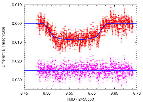
plot    [8.45:8.70] [0.035:-0.01] \
        '$base.model' u (\$1-2455550):2:(\$3*1.45) w err pt 7 ps 0.6 , \
        '$base.curve' u (\$1-2455550):2 w l lt 1 lw 3 lc 3 , \
        '$base.model' u (\$1-2455550):(0.025+\$5):(\$3*1.45) w err pt 7 ps 0.6 lc 4 , \
        0.025 w l lt 1 lw 3 lc 3 

EOF

The output of this plotting script, i.e. the photometry for the transit of the planet HAT-P-13b on the night of 2010 December 27/28 (superimposed with the best-fit light curve model for this event) is then:

---

Back to the examples or the main page.

---